Maranhão Deforestation - Determining Climate Risks with NASA EarthData Cloud

Deforestation of the Amazon Rainforest in Brazil is an ongoing challenge; in this notebook, we’ll use OPERA DIST-HLS data product to study the evolution of vegetation loss due to natural and anthropogenic causes. In particular, we’ll examine deforestation over a period of roughly two years in the state of Maranhão, Brazil.

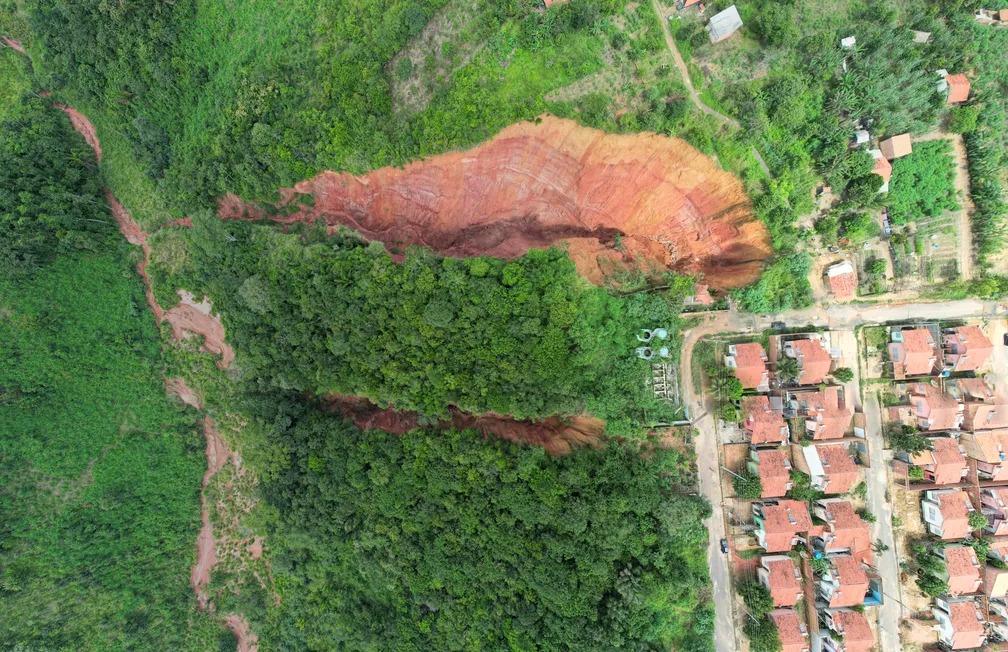
(from https://www.querencianews.com.br/video-de-drone-mostra-cidade-do-maranhao-que-corre-risco-de-desaparecer-por-causa-de-crateras)

Outline of steps for analysis¶

Identifying search parameters (AOI, time-window, endpoint, etc.)
Obtaining search results
Exploring & refining search results
Data-wrangling to produce relevant output

In this case, we’ll assemble a DataFrame to summarize search results, trim down the results to a manageable size, and make an interactive slider to examine the data retrieved.

Preliminary imports¶

from warnings import filterwarnings
filterwarnings('ignore')
import numpy as np, pandas as pd, xarray as xr
import rioxarray as rio
import rasterio

import hvplot.pandas, hvplot.xarray
import geoviews as gv
from geoviews import opts
gv.extension('bokeh')

from pystac_client import Client
from osgeo import gdal
# GDAL setup for accessing cloud data
gdal.SetConfigOption('GDAL_HTTP_COOKIEFILE','~/.cookies.txt')
gdal.SetConfigOption('GDAL_HTTP_COOKIEJAR', '~/.cookies.txt')
gdal.SetConfigOption('GDAL_DISABLE_READDIR_ON_OPEN','EMPTY_DIR')
gdal.SetConfigOption('CPL_VSIL_CURL_ALLOWED_EXTENSIONS','TIF, TIFF')

Convenient utilities¶

These functions could be placed in module files for more developed research projects. For learning purposes, they are embedded within this notebook.

# simple utility to make a rectangle with given center of width dx & height dy
def make_bbox(pt,dx,dy):
    '''Returns bounding-box represented as tuple (x_lo, y_lo, x_hi, y_hi)
    given inputs pt=(x, y), width & height dx & dy respectively,
    where x_lo = x-dx/2, x_hi=x+dx/2, y_lo = y-dy/2, y_hi = y+dy/2.
    '''
    return tuple(coord+sgn*delta for sgn in (-1,+1) for coord,delta in zip(pt, (dx/2,dy/2)))

# simple utility to plot an AOI or bounding-box
def plot_bbox(bbox):
    '''Given bounding-box, returns GeoViews plot of Rectangle & Point at center
    + bbox: bounding-box specified as (lon_min, lat_min, lon_max, lat_max)
    Assume longitude-latitude coordinates.
    '''
    # These plot options are fixed but can be over-ridden
    point_opts = opts.Points(size=12, alpha=0.25, color='blue')
    rect_opts = opts.Rectangles(line_width=0, alpha=0.1, color='red')
    lon_lat = (0.5*sum(bbox[::2]), 0.5*sum(bbox[1::2]))
    return (gv.Points([lon_lat]) * gv.Rectangles([bbox])).opts(point_opts, rect_opts)

# utility to extract search results into a Pandas DataFrame
def search_to_dataframe(search):
    '''Constructs Pandas DataFrame from PySTAC Earthdata search results.
    DataFrame columns are determined from search item properties and assets.
    'asset': string identifying an Asset type associated with a granule
    'href': data URL for file associated with the Asset in a given row.'''
    granules = list(search.items())
    assert granules, "Error: empty list of search results"
    props = list({prop for g in granules for prop in g.properties.keys()})
    tile_ids = map(lambda granule: granule.id.split('_')[3], granules)
    rows = (([g.properties.get(k, None) for k in props] + [a, g.assets[a].href, t])
                for g, t in zip(granules,tile_ids) for a in g.assets )
    df = pd.concat(map(lambda x: pd.DataFrame(x, index=props+['asset','href', 'tile_id']).T, rows),
                   axis=0, ignore_index=True)
    assert len(df), "Empty DataFrame"
    return df

Obtaining search results¶

We’ll focus on an area of interest centered at the geographic longitude-latitude coordinates $(-43.65,^{\circ}, -3.00^{\circ})$ that lies within the state of Maranhão, Brazil. We’ll look at as much data as is available from January 2022 until the end of March 2024.

AOI = make_bbox((-43.65, -3.00), 0.2, 0.2)
DATE_RANGE = "2022-01-01/2024-03-31"

The plot generated below illustrates the AOI; the Bokeh Zoom tool is useful to examine the box on several length scales.

# Optionally plot the AOI
basemap = gv.tile_sources.OSM(padding=0.1, alpha=0.75)
plot_bbox(AOI) * basemap

search_params = dict(bbox=AOI, datetime=DATE_RANGE)
print(search_params)

To execute the search, we define the endpoint URI and instantiate a Client object.

ENDPOINT = 'https://cmr.earthdata.nasa.gov/stac'
PROVIDER = 'LPCLOUD'
COLLECTIONS = ["OPERA_L3_DIST-ALERT-HLS_V1_1"]
search_params.update(collections=COLLECTIONS)
print(search_params)

catalog = Client.open(f'{ENDPOINT}/{PROVIDER}/')
search_results = catalog.search(**search_params)

The search itself is quite fast and yields a few thousand results that can be more easily examined in a Pandas DataFrame.

%%time
df = search_to_dataframe(search_results)
df.info()
df.head()

We clean the DataFrame df in typical ways that make sense:

renaming the eo:cloud_cover column as cloud_cover;
casting the cloud_cover column as floating-point values;
dropping extraneous datetime columns;
casting the datetime column as DatetimeIndex;
setting the datetime column as the Index; and
casting the remaining columns as strings.

df = df.rename(columns={'eo:cloud_cover':'cloud_cover'})
df.cloud_cover = df.cloud_cover.astype(np.float16)
df = df.drop(['start_datetime', 'end_datetime'], axis=1)
df.datetime = pd.DatetimeIndex(df.datetime)
df = df.set_index('datetime').sort_index()
for col in 'asset href tile_id'.split():
    df[col] = df[col].astype(pd.StringDtype())

df.info()

Exploring & refining search results¶

The particular band of the DIST-ALERT data that interests us is the VEG-DIST-STATUS band, so we’ll construct a boolean series c1 that is True whenever the string in the asset column includes VEG-DIST-STATUS as a sub-string. We can also construct a boolean series c2 to filter out rows for which the cloud_cover exceeds 20%.

c1 = df.asset.str.contains('VEG-DIST-STATUS')

c2 = df.cloud_cover<20

If we examine the tile_id column, we can see that a single MGRS tile contains the AOI we specified. As such, all the data indexed in df corresponds to distinct measurements taken from a fixed geographic tile at different times.

df.tile_id.value_counts()

We can combine the information above to reduce the DataFrame to a much shorter sequence of rows. We can also drop the asset and tile_id columns because they will be the same in every row after filtering. We really only need the href column going forward.

df = df.loc[c1 & c2].drop(['asset', 'tile_id', 'cloud_cover'], axis=1)
df.info()

It looks as though there are only 11 rows remaining after filtering the others out. These can be visualized interactively as shown below.

Data-wrangling to produce relevant output¶

df

Each row of the DataFrame is associated with a distinct granule (in this context, a GeoTIFF file produced from an observation made at a given timestamp). We’ll use a loop to assemble a stacked DataArray from the remote files using xarray.concat.

%%time
stack = []
for timestamp, row in df.iterrows():
    data = rio.open_rasterio(row.href).squeeze()
    data = data.rename(dict(x='longitude', y='latitude'))
    del data.coords['band']
    data.coords.update({'time':timestamp})
    data.attrs = dict(description=f"OPERA DIST: VEG-DIST-STATUS", units=None)
    stack.append(data)
stack = xr.concat(stack, dim='time')
stack

As a reminder, for the VEG-DIST-STATUS band, we interpret the raster values as follows:

0: No disturbance
1: First detection of disturbance with vegetation cover change <50%
2: Provisional detection of disturbance with vegetation cover change <50%
3: Confirmed detection of disturbance with vegetation cover change <50%
4: First detection of disturbance with vegetation cover change ≥50%
5: Provisional detection of disturbance with vegetation cover change ≥50%
6: Confirmed detection of disturbance with vegetation cover change ≥50%
7: Finished detection of disturbance with vegetation cover change <50%
8: Finished detection of disturbance with vegetation cover change ≥50%
255 Missing data

By applying np.unique to the stack of rasters, we see that all these 10 distinct values occur somewhere in the data.

np.unique(stack)

We’ll treat the pixels with missing values (i.e., value 255) the same as pixels with no disturbance (i.e., value 0). We could assign the value nan, but that converts the data to float32 or float64 and hence increases the amount of memory required. That is, reassigning 255->0 allows us to ignore the missing values.

stack = stack.where(stack!=255, other=0)

np.unique(stack)

We’ll define a colormap to identify pixels showing signs of disturbance. Rather than assigning different colors to each of the 8 categories, we’ll use RGBA (“red green blue alpha”) values to assign colors with a transparency value. With the colormap defined in the next cell, most of the pixels will be fully transparent. The remaining pixels are red with strictly positive alpha values. The values we really want to see are 3, 6, 7, & 8 (indicating confirmed ongoing disturbance or disturbance that has finished).

# Define a colormap using RGBA values; these need to be written manually here...
COLORS = [
            (255, 255, 255, 0.0),   # No disturbance
            (255,   0,   0, 0.25),  # <50% disturbance, first detection
            (255,   0,   0, 0.25),  # <50% disturbance, provisional
            (255,   0,   0, 0.50),  # <50% disturbance, confirmed, ongoing
            (255,   0,   0, 0.50),  # ≥50% disturbance, first detection
            (255,   0,   0, 0.50),  # ≥50% disturbance, provisional
            (255,   0,   0, 1.00),  # ≥50% disturbance, confirmed, ongoing
            (255,   0,   0, 0.75),  # <50% disturbance, finished
            (255,   0,   0, 1.00),  # ≥50% disturbance, finished
         ]

Finally, we’re ready to produce visualizations using the array stack.

We define view as a subset of stack that uses skips steps pixels in each direction to speed rendering (change to steps=1 or steps=None when ready to plot at full resolution).
We define dictionaries image_opts and layout_opts to control arguments to pass to hvplot.image.
The result, when plotted, is an interactive plot with a slider that allows us to view specific time slices of the data.

steps = 100
subset=slice(0,None,steps)
view = stack.isel(longitude=subset, latitude=subset)

image_opts = dict(
                    x='longitude',
                    y='latitude',
                    cmap=COLORS,
                    colorbar=False,
                    clim=(-0.5,8.5),
                    crs = stack.rio.crs,
                    tiles=gv.tile_sources.ESRI,
                    tiles_opts=dict(alpha=0.1, padding=0.1),
                    project=True,
                    rasterize=True,
                    widget_location='bottom',
                 )

layout_opts = dict(
                    title = 'Maranhão \nDisturbance Alerts',
                    xlabel='Longitude (°)',ylabel='Latitude (°)',
                    fontscale=1.25,
                    frame_width=500,
                    frame_height=500,
                  )

view.hvplot.image(**image_opts, **layout_opts)

The slider here allows us to see a trend of increasing deforestation over the course of two years. The earlier rasters have red pixels sparsely distributed over the region, whereas the later rasters have far more red pixels (indicating damaged vegetation). It is a simple matter to use the array stack to count pixels in each category and to assemble quantitative measures of deforestation.

4. Case Studies

The Bhakra Nangal Dam & Gobind Sagar Reservoir

4. Los Casos Prácticos

Plantilla para el uso de del servicio cloud ofrecido por EarthData