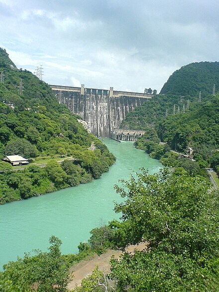
The Bhakra Nangal dam was opened in 1963 in India. The dam forms the Gobind Sagar reservoir and provides irrigation to 10 million acres in the neighboring states of Punjab, Haryana, and Rajasthan. We can use OPERA DSWx data to observe fluctuations in water levels over long time periods.
Outline of steps for analysis
- Identifying search parameters
- AOI, time-window
- Endpoint, Provider, catalog identifier (“short name”)
- Obtaining search results
- Instrospect, examine to identify features, bands of interest
- Wrap results into a DataFrame for easier exploration
- Exploring & refining search results
- Identify granules of highest value
- Filter extraneous granules with minimal contribution
- Assemble relevant filtered granules into DataFrame
- Identify kind of output to generate
- Data-wrangling to produce relevant output
- Download relevant granules into Xarray DataArray, stacked appropriately
- Do intermediate computations as necessary
- Assemble relevant data slices into visualization
Preliminary imports
from warnings import filterwarnings
filterwarnings('ignore')
import numpy as np, pandas as pd, xarray as xr
import rioxarray as rio
import rasterio
# Imports for plotting
import hvplot.pandas, hvplot.xarray
import geoviews as gv
from geoviews import opts
gv.extension('bokeh')# STAC imports to retrieve cloud data
from pystac_client import Client
from osgeo import gdal
# GDAL setup for accessing cloud data
gdal.SetConfigOption('GDAL_HTTP_COOKIEFILE','~/.cookies.txt')
gdal.SetConfigOption('GDAL_HTTP_COOKIEJAR', '~/.cookies.txt')
gdal.SetConfigOption('GDAL_DISABLE_READDIR_ON_OPEN','EMPTY_DIR')
gdal.SetConfigOption('CPL_VSIL_CURL_ALLOWED_EXTENSIONS','TIF, TIFF')Convenient utilities
# simple utility to make a rectangle with given center of width dx & height dy
def make_bbox(pt,dx,dy):
    '''Returns bounding-box represented as tuple (x_lo, y_lo, x_hi, y_hi)
    given inputs pt=(x, y), width & height dx & dy respectively,
    where x_lo = x-dx/2, x_hi=x+dx/2, y_lo = y-dy/2, y_hi = y+dy/2.
    '''
    return tuple(coord+sgn*delta for sgn in (-1,+1) for coord,delta in zip(pt, (dx/2,dy/2)))
# simple utility to plot an AOI or bounding-box
def plot_bbox(bbox):
'''Given bounding-box, returns GeoViews plot of Rectangle & Point at center
+ bbox: bounding-box specified as (lon_min, lat_min, lon_max, lat_max)
Assume longitude-latitude coordinates.
'''
# These plot options are fixed but can be over-ridden
point_opts = opts.Points(size=12, alpha=0.25, color='blue')
rect_opts = opts.Rectangles(line_width=0, alpha=0.1, color='red')
lon_lat = (0.5*sum(bbox[::2]), 0.5*sum(bbox[1::2]))
return (gv.Points([lon_lat]) * gv.Rectangles([bbox])).opts(point_opts, rect_opts)# utility to extract search results into a Pandas DataFrame
def search_to_dataframe(search):
'''Constructs Pandas DataFrame from PySTAC Earthdata search results.
DataFrame columns are determined from search item properties and assets.
'asset': string identifying an Asset type associated with a granule
'href': data URL for file associated with the Asset in a given row.'''
granules = list(search.items())
assert granules, "Error: empty list of search results"
props = list({prop for g in granules for prop in g.properties.keys()})
tile_ids = map(lambda granule: granule.id.split('_')[3], granules)
rows = (([g.properties.get(k, None) for k in props] + [a, g.assets[a].href, t])
for g, t in zip(granules,tile_ids) for a in g.assets )
df = pd.concat(map(lambda x: pd.DataFrame(x, index=props+['asset','href', 'tile_id']).T, rows),
axis=0, ignore_index=True)
assert len(df), "Empty DataFrame"
return df# utility to remap pixel values to a sequence of contiguous integers
def relabel_pixels(data, values, null_val=255, transparent_val=0, replace_null=True, start=0):
"""
This function accepts a DataArray with a finite number of categorical values as entries.
It reassigns the pixel labels to a sequence of consecutive integers starting from start.
data: Xarray DataArray with finitely many categories in its array of values.
null_val: (default 255) Pixel value used to flag missing data and/or exceptions.
transparent_val: (default 0) Pixel value that will be fully transparent when rendered.
replace_null: (default True) Maps null_value->transparent_value everywhere in data.
start: (default 0) starting range of consecutive integer values for new labels.
The values returned are:
new_data: Xarray DataArray containing pixels with new values
relabel: dictionary associating old pixel values with new pixel values
"""
new_data = data.copy(deep=True)
if values:
values = np.sort(np.array(values, dtype=np.uint8))
else:
values = np.sort(np.unique(data.values.flatten()))
if replace_null:
new_data = new_data.where(new_data!=null_val, other=transparent_val)
values = values[np.where(values!=null_val)]
n_values = len(values)
new_values = np.arange(start=start, stop=start+n_values, dtype=values.dtype)
assert transparent_val in new_values, f"{transparent_val=} not in {new_values}"
relabel = dict(zip(values, new_values))
for old, new in relabel.items():
if new==old: continue
new_data = new_data.where(new_data!=old, other=new)
return new_data, relabelThese functions could be placed in module files for more developed research projects. For learning purposes, they are embedded within this notebook.
Identifying search parameters
For coordinates of the dam, we’ll use . We’ll also look for a full calendar year’s worth of data between April 1, 2023 and April 1, 2024.
AOI = make_bbox((76.46, 31.42), 0.2, 0.2)
DATE_RANGE = "2023-04-01/2024-04-01"
# Optionally plot the AOI
basemap = gv.tile_sources.OSM(alpha=0.5, padding=0.1)
plot_bbox(AOI) * basemapsearch_params = dict(bbox=AOI, datetime=DATE_RANGE)
print(search_params)Obtaining search results
We’re going to look for OPERA DSWx data products, so we define the ENDPOINT, PROVIDER, and COLLECTIONS as follows (these values are occasionally modified, so some searching through NASA’s Earthdata Search website may be necessary).
ENDPOINT = 'https://cmr.earthdata.nasa.gov/stac'
PROVIDER = "POCLOUD"
COLLECTIONS = ["OPERA_L3_DSWX-HLS_V1_1.0"]
# Update the dictionary opts with list of collections to search
search_params.update(collections=COLLECTIONS)
print(search_params)
%%time
catalog = Client.open(f'{ENDPOINT}/{PROVIDER}/')
search_results = catalog.search(**search_params)Having executed the search, the results can be perused in a DataFrame.
%%time
df = search_to_dataframe(search_results)
df.head()
We’ll clean the DataFrame df by renaming the eo:cloud_cover column, dropping the extra datetime columns, converting the datatypes sensibly, and setting the index.
df = df.rename(columns={'eo:cloud_cover':'cloud_cover'})
df.cloud_cover = df.cloud_cover.astype(np.float16)
df = df.drop(['start_datetime', 'end_datetime'], axis=1)
df = df.convert_dtypes()
df.datetime = pd.DatetimeIndex(df.datetime)
df = df.set_index('datetime').sort_index()
df.info()
df.head()At this stage, the DataFrame of search results has over two thousand rows. Let’s trim that down.
Exploring & refining search results
We’ll filter the rows of df to capture only granules captured with less than 10% cloud cover and the B01_WTR band of the DSWx data.
c1 = df.cloud_cover<10
c2 = df.asset.str.contains('B01_WTR')
df = df.loc[c1 & c2]
df.info()We can count all the distinct entries of the tile_id column and. find that there’s only one (T43RFQ). This means that the AOI specified lies strictly inside a single MGRS tile and that all granules found will be associated with that particular geographic tile.
df.tile_id.value_counts()We’ve reduced the total number of granules to a little over fifty. Let’s use these to produce a visualization.
Data-wrangling to produce relevant output
As we’ve seen several times now, we’ll stack the two-dimensional arrays from the GeoTIFF files listed in df.href into a three-dimensional DataArray; we’ll use the identifier stack to label the result.
%%time
stack = []
for timestamp, row in df.iterrows():
    data = rio.open_rasterio(row.href).squeeze()
    data = data.rename(dict(x='longitude', y='latitude'))
    del data.coords['band']
    data.coords.update({'time':timestamp})
    data.attrs = dict(description=f"OPERA DIST: VEG-DIST-STATUS", units=None)
    stack.append(data)
stack = xr.concat(stack, dim='time')
stack
We can see the pixel values that actually occur in the array stack using the NumPy unique function.
np.unique(stack)As a reminder, according to the DSWx product specification, the meanings of the raster values are as follows:
- 0: Not Water—any area with valid reflectance data that is not from one of the other allowable categories (open water, partial surface water, snow/ice, cloud/cloud shadow, or ocean masked).
- 1: Open Water—any pixel that is entirely water unobstructed to the sensor, including obstructions by vegetation, terrain, and buildings.
- 2: Partial Surface Water—an area that is at least 50% and less than 100% open water (e.g., inundated sinkholes, floating vegetation, and pixels bisected by coastlines).
- 252: Snow/Ice.
- 253: Cloud or Cloud Shadow—an area obscured by or adjacent to cloud or cloud shadow.
- 254: Ocean Masked—an area identified as ocean using a shoreline database with an added margin.
- 255: Fill value (missing data).
Notice that the value 254—ocean masked—does not occur in this particular collection of rasters because this particular region is far away from the coast.
To clean up the data (in case we want to use a colormap), let’s reassign the pixel values with our utility function relabel_pixels. This time, let’s keep the “no data” (255) values so we can see where data is missing.
stack, relabel = relabel_pixels(stack, values=[0,1,2,252,253,255], replace_null=False)We can execute np.unique again to ensure that the data has been modified as intended.
np.unique(stack)Let’s now assign a colormap to help visualize the raster images. In this instance, the colormap uses several distinct colors with full opacity and black, partially transparent pixels to indicate missing data.
# Define a colormap using RGBA values; these need to be written manually here...
COLORS = {
0: (255, 255, 255, 0.0),  # Not Water
1: (  0,   0, 255, 1.0),  # Open Water
2: (180, 213, 244, 1.0),  # Partial Surface Water
3: (  0, 255, 255, 1.0),  # Snow/Ice
4: (175, 175, 175, 1.0),  # Cloud/Cloud Shadow
5: (  0,   0, 0, 0.5),    # Missing
}
We’re ready to plot the data.
- We define suitable options in the dictionaries
image_optsandlayout_opts. - We construct an object
viewthat consists of slices extracted fromstackby subsampling everystepspixels (reducestepsto1orNoneto view the rasters at full resolution).
image_opts = dict(
                    x='longitude',
                    y='latitude',
                    cmap = list(COLORS.values()),
                    colorbar=False,
                    tiles = gv.tile_sources.OSM,
                    tiles_opts=dict(padding=0.05, alpha=0.25),
                    project=True,
                    rasterize=True,
                    framewise=False,
                    widget_location='bottom',
                 )

layout_opts = dict(
                    title = 'Bhakra Nangal Dam, India - water extent over a year',
                    xlabel='Longitude (degrees)',
                    ylabel='Latitude (degrees)',
                    fontscale=1.25,
                    frame_width=500,
                    frame_height=500
                   )
steps = 100
subset = slice(0,None,steps)
view = stack.isel(longitude=subset, latitude=subset)
view.hvplot.image( **image_opts, **layout_opts)The visualization above may take a wile to update (depending on the choice of steps). It does provide a way to see the water accumulation over a period of a year. There are a number of slices in which a lot of data is missing, so some care is required to interpret those time slices.