Coordinate Reference Systems

Later in this tutorial, we’ll extract & analyze geospatial datasets from spatio-temporal asset catalogs (usually called STACs). In particular, this means we need to specify precisely a geographical region—usually called an area of interest or AOI—and a time window that respectively describe where & when a relevant event occurred (e.g., a flood, a wild fire, etc.). That is, both the spatial location and the time period of interest need to be expressed unambiguously to search for relevant data.

Geospatial datasets—whether it be raster data or vector data (as described in the next two notebooks)—need to be represented using a chosen Coordinate Reference Systems (CRS). In the context of Geographic Information Systems (GIS), a CRS is a mathematical framework that defines how geographical features & locations on the Earth’s surface are associated with numerical coordinates (tuples in two or three dimensions). A coordinate representation is needed to compute geometric quantities (e.g., distances/lengths, angles, areas, volumes, etc.) accurately for geospatial analysis.

The present notebook summarizes the main framework we’ll use: the Military Grid Reference System (MGRS). This system is built using the Universal Transverse Mercator (UTM), a particular projected coordinate reference system. To understand all these pieces, we also need to know a few basic facts about Geographic Coordinate System (GCS) that employ on latitude-longitude coordinates.

An aside about timestamps¶

Let’s first consider the problem of specifying a time interval unambiguously—we encounter challenges doing so in ordinary contexts (e.g., trying to schedule a call between people residing in different time zones). Earth scientists generally use UTC (Coordinated Universal Time) when recording timestamps associated with measurements or observations to avoid time-zone difficulties. This is the case for all the NASA data products we’ll work with. There are subtle questions about the degree of precision with which a timestamp is given (e.g., within days, hours, minutes, seconds, milliseconds, and so on); regardless, using UTC is a standard way of representing points in time (or a time window between two timestamps) without ambiguity.

Geographic Coordinate Systems¶

Most people are familiar with the Global Positioning System (GPS) that uses a Geographic Coordinate System (GCS) to represent locations on the Earth’s surface. Geographic coordinate systems are implicitly based on spherical coordinate systems in which points on the surface of a sphere are determined by two angular values called latitude & longitude. Of course, the Earth is not actually spherical. Its shape is better modelled by an ellipsoid or an oblate spheroid (although there are still corrections to make accounting for topography and other surface features). The World Geodetic System refers to an agreed-upon standard model of the Earth that is used for applications in geodesy, cartography, and satellite navigation. The current version of this standard is WGS84 which includes a geodetic datum (a mathematical description of a reference ellipsoid together with a reference point on the surface and an oriented, Earth-centered, Earth-fixed coordinate system), an associated Earth Gravitational Model (EGM) and a World Magnetic Model (WMM). We do not need to concern ourselves with the specifics of WGS84 other than to acknowledge that this standard underlies any GCS using latitude-longitude coordinates.

Here are some relevant facts about GCS latitude-longitude coordinates we’ll rely on throughout this tutorial:

• The latitude (ϕ) of a point $P$ on the surface of a sphere represents the angle between equatorial plane and a line segment between $P$ and $O$, the sphere’s center. Thus, the latitude of any point on the equator is $0^\circ$, the latitude at the upper (north) pole is $+90^\circ$ and the latitude at the lower (south) pole is $-90^\circ$.
• The longitude (λ) of a point $P$ on the surface of a sphere is the angle extended between two planes: the first plane contains both poles and an anchor point on the sphere’s surface; and the second plane contains the point P and both poles. The typical choice for an anchor point on the Earth’s surface used in GCS is Greenwich, England. The great circle passing through Greenwich and the poles is called the prime meridian. Any points strictly to the west of Greenwich have negative longitude values (between $-180^\circ$ and $0^\circ$) whereas points strictly to the east of Greenwich have positive longitude values (between $0^\circ$ and $180^\circ$).
• Latitude and longitude coordinates are usually expressed in angular units of degrees (denoted ${}^\circ$). When more precision is required, a degree is divided up into 60 minutes (denoted ${}'$) each of which can be divided further into 60 seconds (denoted ${}"$). Decimal representations of latitude-longitude pairs are used in many places, but we may encounter both conventions to represent coordinates.
• Great circles through the poles are referred to as meridians. Meridians have a fixed longitude value.
• Circles in planes parallel to the equatorial plane are referred to as parallels. Parallels have a fixed latitude value.
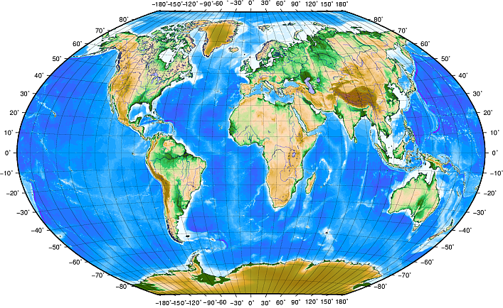
• At the Earth’s equator, one second of longitude corresponds to roughly 30 meters. However, there is a nonlinear relationship between differences in latitude-longitude coordinates and distances on the Earth’s surface (and hence distortions in other geometrical properties). For instance, let’s consider two angular regions of “width” $1^\circ$ in longitude and “height” $1^\circ$ in latitude (aligned with the latitude-longitude axes). On a map using GCS coordinates, those two regions would have the same area; however, the corresponding areas on the Earth’s surface would differ. In particular, whichever patch is closer to the equator would have a greater surface area. Specifically, closer to the poles, the lines of constant longitude and latitude are closer together, so areas get compressed (this is a feature of any GCS).

Projected coordinate reference systems¶

Cartographers and geographers prefer working with maps on which the distances measured between points on the map are approximately proportional to actual physical distances. This is decidedly not the case for maps using GCS latitude-longitude coordinates

A more practical approach for geographical purposes is to use a projected coordinate reference system instead. That is, use a CRS whose coordinates are found using a map projection that projects points in a fixed region on the Earth’s curved surface to a flat two-dimensional plane. Such a transformation necessarily distorts the Earth’s curved surface but, locally, geometric distances between points on the plane are approximately proportional to actual distances. Thus, the coordinates in a projected coordinate system are typically expressed in units of length (e.g., metres). Projections involve compromises in that different projections more reliably represent certain geometric properties—shape, area, distance, etc.—more accurately.

Universal Transverse Mercator (UTM) coordinates¶

The Universal Transverse Mercator (UTM) is a particular projected coordinate reference system. These coordinate values are typically referred to as easting and northing (referring to distances east and north respectively from the origin in some locally flattened plane).

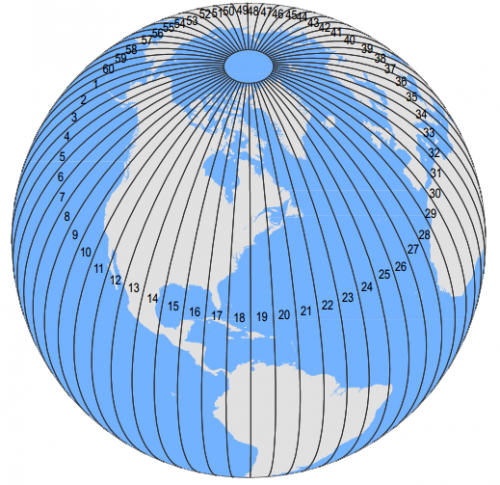
• The UTM CRS divides the world map into 60 zones of width $6^\circ$ in longitude that extend between $-80^\circ$ & $+84^\circ$ latitude. The UTM zones are numbered 1 to 60, starting at the antimeridian (i.e., zone 1 at $-180^\circ$ longitude) and progressing east back to the antemeridian (i.e., zone 60 at $+180^\circ$ longitude).
• The origin within each UTM zone is on the equator at the zone’s central meridian.
• There are formulas to convert from latitude-longitude GCS coordinates to UTM easting-northing as well as formulas to do the opposite. We need not concern ourselves with those details in this tutorial other than to know that software routines implement those formulas to effect those transformations.
• The position of a point in UTM coordinates usually involves specifying two positive values for the easting & northing coordinates as well as the UTM zone number. The easting value is the number of meters east of the zones central meridian and the northing value is the number of meters north of the equator. To avoid using negative coordinates, a false northing value of $10,000,000\,\mathrm{m}$ to the northing coordinate and a false easting value of $500,000\,\mathrm{m}$ is added to the easting coordinate.

A note on Coordinate Reference Systems¶

There are, in principle, infinitely many coordinate reference systems that associate locations on the Earth’s surface with two- or three-dimensional tuples of numbers (coordinates). To characterize a number of practical CRSs concisely, the European Petroleum Survey Group (EPSG) maintains the public EPSG registry. A CRS is assigned a code between 1024 and 32767 along with a standard machine-readable well-known text (WKT) representation.

Here are some important examples of EPSG CRS codes:

• EPSG:4326 is the CRS using standard latitude-longitude coordinates based on the WGS84 geodetic model as used for GPS & navigation.
• EPSG:3857 is the Web Mercator projected CRS used in, e.g., Google Maps & OpenStreetMaps due to its convenience for rendering & for straight-line navigation. It does distort distances significantly closer to the poles.
• EPSG:32610 is a particular projected UTM CRS. Similar UTM projected CRSs have a code of the form EPSG:326XY; the digits 326 indicate a UTM projected CRS valid in the Northern hemisphere. The last two digits—10 in this instance—identify a particular UTM zone between 01 and 60.
• EPSG:32710 is also a particular projected UTM CRS. The digits 327 indicate a UTM projected CRS valid in the Southern hemisphere & the last two digits—again, 10 in this instance—identify a particular UTM zone between 01 and 60.

From a mathematical viewpoint, an EPSG code is a compact identifier connecting to standardized sets of equations, parameters, and rules.

Military Grid Reference System (MGRS)¶

The last convention we need to know is the Military Grid Reference System (MGRS). The MGRS is used primarily by NATO militaries to identify Earth locations. The MGRS is not a CRS; rather it is a geocoordinate standard layered on top of other CRSs. Away from the polar region, the MGRS uses the Universal Transverse Mercator (UTM) coordinate system; near the poles, it uses the Universal Polar Stereographic (UPS) coordinate system instead. In both cases, MGRS relies on projected CRSs based on the WGS84 model for accurate spatial representations.

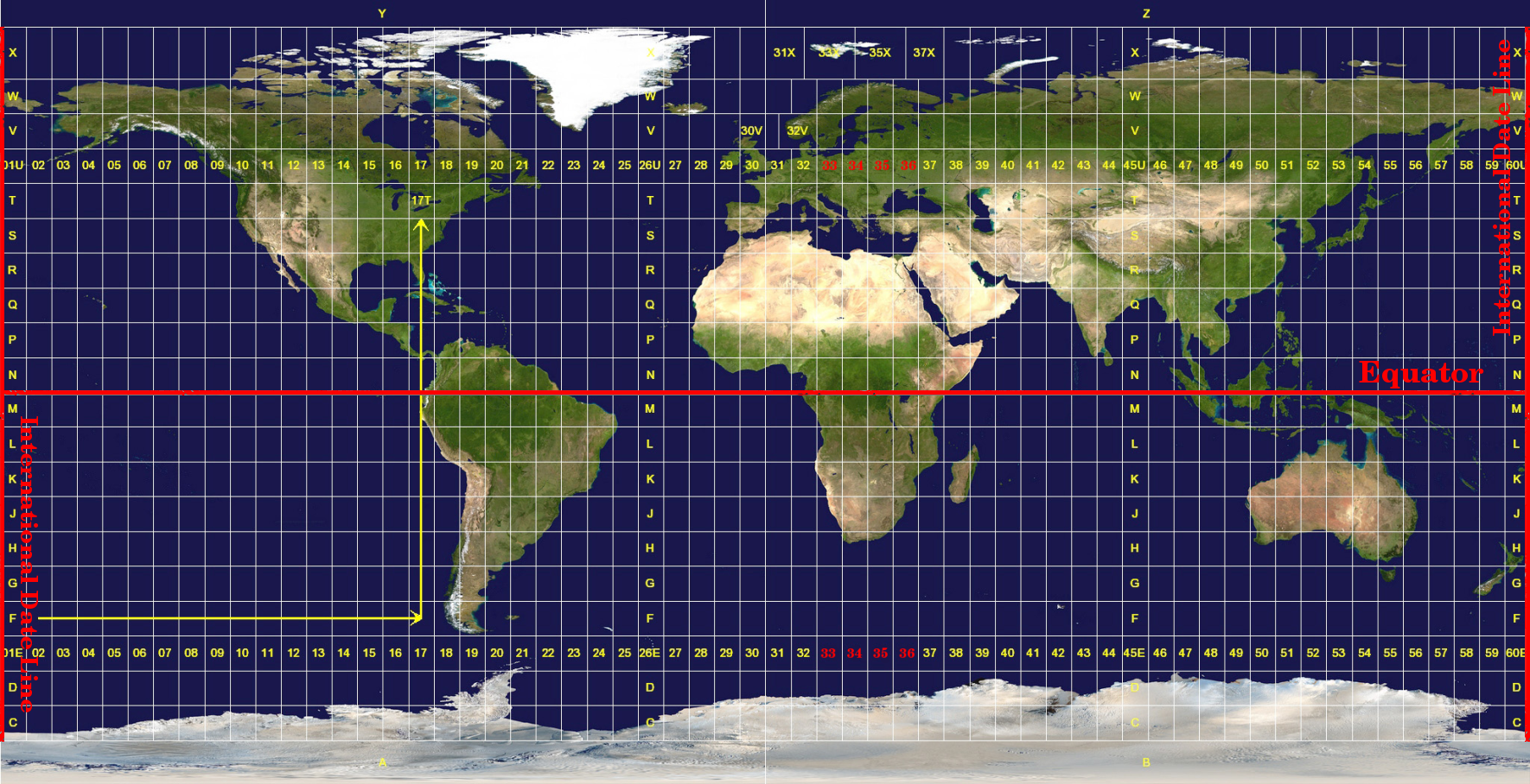
The MGRS system uses UTM zones as a basis for its grid. Remember, the UTM system divides the Earth’s surface into 60 zones, each of width $6^{\circ}$ longitude, extending from $-80^\circ$ to $+84^\circ$. Each UTM zone is divided into 20 horizontal latitude bands each of of height $8^\circ$ latitude; these latitude bands are labeled C through X (excluding the letters I and O to avoid confusion with 1 & 0 respectively). These first two labels constitute a grid-zone designator (GZD). These 1,200 MGRS grid-zones are further subdivided into tiles of area $(100\,\mathrm{km}\times100\,\mathrm{km})$; these smaller tiles are labelled by column and row within each GZD. For instance, the tile identifier 10TEM indicates that the tile in question is in UTM zone 10 in the horizontal band T. Within that GZD, there is a grid of tiles and the one with column index E and row index M is the tile in question. These tile labels help identify the coordinates of the corners of a square region associated with a satellite image as well as the projected coordinate system used to map points on the Earth’s surface to the projected tile coordinates.

In essence, MGRS is a refinement of the UTM coordinate system, designed for easier readability and communication in military and navigation applications. The system’s hierarchical structure—from UTM zone to latitude band to 100 km grid squares, and finally down to precise easting and northing coordinates—enables efficient referencing without needing large numeric coordinates.